


It seems like everyone is releasing some cool model right now, so why not join the fun? Here at Count Bayesie we are introducing a new model unlike anything you’ve seen before: Linear Diffusion! A diffusion model that uses only linear models as its components (and currently works best with a very simple “language” and MNIST digits as images).
You can get the model and code on Github right now. If you’d like to learn more about Linear Diffusion, read on!
Here is a basic overview of Linear Diffusion’s architecture:

Visualization of the modifications to the standard diffusion model used by Linear Diffusion.
Why Linear Diffusion you might ask? As you may know, I’m a big believer in the power of linear models, and have many times argued one should never start any ambitious project without first building a linear model to see if you can get some decent performance from that. Only after a simple model shows promise should you add complexity. Surely this wisdom must fail when talking about state of the art models such as Stable Diffusion and Dall-E 2 right!? Is it even possible to have a linear diffusion model?
That’s what I wanted to find out! To make this problem a bit easier for a linear model to figure out I’ve constrained the problem space a bit including:
-
Statements in the language are limited to just the string representations of the digits 0-9
-
The images are the MNIST digits
Given these constraints, it turns out we can build such a model and can get some surprisingly good outputs from it! Here’s an example of Linear Diffusion’s responses to various prompts:

Digits generated from Linear Diffusion
While certainly not an “astronaut riding a horse”, I personally think these are pretty impressive results for what is ultimately a linear model. As an added bonus, working through building Linear Diffusion provides a pretty good, high level overview of what real diffusion models are doing!
Before we can build our Linear Diffusion model, we first need to understand what diffusion models are doing under the hood. It’s difficult to understate the complexity of these models in practice, so be advised: we are looking at this model from an extremely high level of abstraction. However even this high level of abstraction will allow us to map state of the art diffusion architectures to an implementation using only linear models.
Goal: Generating Images from a Text Description
Let’s be clear about what our final goal is: We want to provide our model with a text description of what we want to see, and have the model return a generated image matching that description. For example we might enter “A salami sandwich” and hope to get an image like this out of Stable Diffusion:
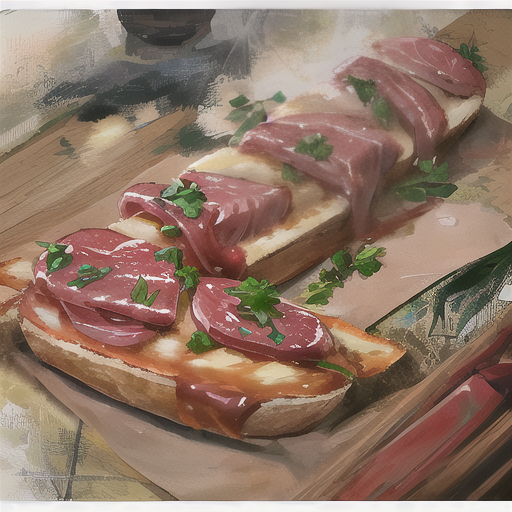
How in the world could a model figure this out?
Most diffusion models we’re familiar with allow you to enter arbitrary text, however for our simple model we’ll limit our language to statements representing digits 0-9. So if we enter ‘“5” we might get an image like this:

A trained Linear Diffusion model was fed only the string “5” and output this image!
Here’s a very quick summary of how these models achieve this goal: diffusion models learn to de-noise a noisy image in a way that agrees with the text describing the image. Then we ask the trained model to de-noise pure noise in a way that agrees with the text description and poof! we have a novel image generated by the model!
Now let’s step through this process a bit more slowly.
A Map for Training and Prediction
It can be useful to visualize our journey, and step through this process using a visualization as our map. Even at a high level of abstraction, diffusion models have a lot of moving parts! Here is a visualization of how training and prediction works for a diffusion model:

The basic journey through a diffusion model
With this guide handy let’s step through the process!
We start with training data that includes images and descriptions of those images. The first two parts of this model happen essentially in parallel: text embedding and image encoding
1a. Text Embedding
We see in part 1a that we take our original text description and then create a vector embedding from this. Typically in diffusion models this will involve not only very sophisticated language models such as an LSTM or Transformer, but also involve an additional step of aligning the text embedding with the image encoding /embedding. This way, in the latent text space we’re defining, text that describes visually similar events will near each other.
In our Linear Diffusion we will simply one-hot encode our digit strings, and we won’t worry about making sure these text embeddings are close to our images embeddings.
1b. Image Encoding
At the same time as we do our text embedding, in step 1b we also encode our image. This serves two purposes. First it compresses our image tremendously, making all the models we’ll need later on much smaller (which is good because in practice diffusion models are gigantic as is!) Additionally, as we’ll see when we step through the implementation of linear diffusion, this embedding does help us to capture some information about the space of images in general, driving even random noise in the encoding space to look like real images when decoded. The images projected onto this embedding/encoding space are sometimes referred to as “latents”, since they are a latent representation of the image.
Real diffusion models typically us a Variational Autoencoder (VAE) for this step, Linear Diffusion will use Principal Component Analysis (PCA), a linear projection of our original data onto orthogonal vectors.
1b (continued). Adding noise to our image encoding
This is one of the most conceptually important steps of the process. We’re going to add noise to our image encoding and that same noise will be what we are trying to predict at a later step. The basic idea is: if we can predict the noise, then we can remove it.
For most Diffusion Models this process is fairly complex, involving adding progressively more or less noise to an image according to a training schedule. Often times information about how much noise is added to the embedding is included in the vector fed to the denoising model.
In Linear Diffusion we’ll simply be adding noise by sampling from a standard Normal distribution.
2. Concatenating the embeddings
This is step is fairly straightforward: the input to our denoising model is going to be the combination of both the text embedding and the noisy image embedding. The idea is that the denoising model will use information from the text embeddings to help it figure out where the noise might be in the image embedding.
3. The Denoising Model
This is the part of the diffusion model that really makes a diffusion model. In this stage we’re going to use all the information we have so far to attempt to predict the noise we’ve added to the image encoding. Our target at this stage is the very noise vector we used to add noise to our image encoding.
The denoising model for most Diffusion Models is a Denoising UNET which is a very sophisticated neural network for processing image data. Linear Diffusion will, of course, be using Linear Regression for this stage. However we will be adding interaction terms to give our model a bit of help in this ambitious task.
At this stage we are done with the training of the model. It’s helpful to also understand how we can go from here to predicting the original image. Understanding this will aid in understanding how this model can generate images from nothing.
4. Subtracting the noise
If we want to reconstruct the original image, the first step in the process is to subtract the noise from the noisy image embedding, leaving us with, if we estimated the noise correctly, the original embedding.
Linear Diffusion will just literally subtract the estimated noise from the embedding, but for real diffusion models the process can very closely mirror the training process of a neural net itself. Diffusion models will typically only subtract out a fraction of the estimated noise, run the new slightly denoised embedding back through the denoiser, and then apply that estimated noise. This process will be repeated multiple times until the final image is produced.
5. Finally, decoding the latent, denoised image embedding
The last step is essentially the same for Linear Diffusion and typical diffusion models: we just take our encoder and run it backwards (or we could learn the decoder separate) and project our latent image back into a full sized image!
A fascinating model if you ask me but: how do we generate images from this?
A Map for Image Generation
The visual guide for generating images given a text prompt requires just a few minor modification to our original model:

The major difference here is that we start with noise rather than a latent image, then “denoise