


This is not an officially supported Google product.
Varun Godbole†, George E. Dahl†, Justin Gilmer†, Christopher J. Shallue‡, Zachary Nado†
† Google Research, Brain Team
‡ Harvard University
- Who is this document for?
- Why a tuning playbook?
- Guide for starting a new project
- A scientific approach to improving model performance
- Determining the number of steps for each training run
- Additional guidance for the training pipeline
- FAQs
- Acknowledgments
- Citing
- Contributing
This document is for engineers and researchers (both individuals and teams)
interested in maximizing the performance of deep learning models. We assume
basic knowledge of machine learning and deep learning concepts.
Our emphasis is on the process of hyperparameter tuning. We touch on other
aspects of deep learning training, such as pipeline implementation and
optimization, but our treatment of those aspects is not intended to be complete.
We assume the machine learning problem is a supervised learning problem or
something that looks a lot like one (e.g. self-supervised). That said, some of
the prescriptions in this document may also apply to other types of problems.
Currently, there is an astonishing amount of toil and guesswork involved in
actually getting deep neural networks to work well in practice. Even worse, the
actual recipes people use to get good results with deep learning are rarely
documented. Papers gloss over the process that led to their final results in
order to present a cleaner story, and machine learning engineers working on
commercial problems rarely have time to take a step back and generalize their
process. Textbooks tend to eschew practical guidance and prioritize fundamental
principles, even if their authors have the necessary experience in applied work
to provide useful advice. When preparing to create this document, we couldn’t
find any comprehensive attempt to actually explain how to get good results with
deep learning. Instead, we found snippets of advice in blog posts and on social
media, tricks peeking out of the appendix of research papers, occasional case
studies about one particular project or pipeline, and a lot of confusion. There
is a vast gulf between the results achieved by deep learning experts and less
skilled practitioners using superficially similar methods. At the same time,
these very experts readily admit some of what they do might not be
well-justified. As deep learning matures and has a larger impact on the world,
the community needs more resources covering useful recipes, including all the
practical details that can be so critical for obtaining good results.
We are a team of five researchers and engineers who have worked in deep learning
for many years, some of us since as early as 2006. We have applied deep learning
to problems in everything from speech recognition to astronomy, and learned a
lot along the way. This document grew out of our own experience training neural
networks, teaching new machine learning engineers, and advising our colleagues
on the practice of deep learning. Although it has been gratifying to see deep
learning go from a machine learning approach practiced by a handful of academic
labs to a technology powering products used by billions of people, deep learning
is still in its infancy as an engineering discipline and we hope this document
encourages others to help systematize the field’s experimental protocols.
This document came about as we tried to crystalize our own approach to deep
learning and thus it represents the opinions of the authors at the time of
writing, not any sort of objective truth. Our own struggles with hyperparameter
tuning made it a particular focus of our guidance, but we also cover other
important issues we have encountered in our work (or seen go wrong). Our
intention is for this work to be a living document that grows and evolves as our
beliefs change. For example, the material on debugging and mitigating training
failures would not have been possible for us to write two years ago since it is
based on recent results and ongoing investigations. Inevitably, some of our
advice will need to be updated to account for new results and improved
workflows. We do not know the optimal deep learning recipe, but until the
community starts writing down and debating different procedures, we cannot hope
to find it. To that end, we would encourage readers who find issues with our
advice to produce alternative recommendations, along with convincing evidence,
so we can update the playbook. We would also love to see alternative guides and
playbooks that might have different recommendations so we can work towards best
practices as a community. Finally, any sections marked with a 🤖 emoji are places
we would like to do more research. Only after trying to write this playbook did
it become completely clear how many interesting and neglected research questions
can be found in the deep learning practitioner’s workflow.
Many of the decisions we make over the course of tuning can be made once at the
beginning of a project and only occasionally revisited when circumstances
change.
Our guidance below makes the following assumptions:
- Enough of the essential work of problem formulation, data cleaning, etc. has
already been done that spending time on the model architecture and training
configuration makes sense. - There is already a pipeline set up that does training and evaluation, and it
is easy to execute training and prediction jobs for various models of
interest. - The appropriate metrics have been selected and implemented. These should be
as representative as possible of what would be measured in the deployed
environment.
Summary: When starting a new project, try to reuse a model that already
works.
- Choose a well established, commonly used model architecture to get working
first. It is always possible to build a custom model later. - Model architectures typically have various hyperparameters that determine
the model’s size and other details (e.g. number of layers, layer width, type
of activation function).- Thus, choosing the architecture really means choosing a family of
different models (one for each setting of the model hyperparameters). - We will consider the problem of choosing the model hyperparameters in
Choosing the initial configuration
and
A scientific approach to improving model performance.
- Thus, choosing the architecture really means choosing a family of
- When possible, try to find a paper that tackles something as close as
possible to the problem at hand and reproduce that model as a starting
point.
Summary: Start with the most popular optimizer for the type of problem at
hand.
- No optimizer is the “best” across all types of machine learning problems and
model architectures. Even just
comparing the performance of optimizers is a difficult task.
🤖 - We recommend sticking with well-established, popular optimizers, especially
when starting a new project.- Ideally, choose the most popular optimizer used for the same type of
problem.
- Ideally, choose the most popular optimizer used for the same type of
- Be prepared to give attention to *all* hyperparameters of the
chosen optimizer.- Optimizers with more hyperparameters may require more tuning effort to
find the best configuration. - This is particularly relevant in the beginning stages of a project when
we are trying to find the best values of various other hyperparameters
(e.g. architecture hyperparameters) while treating optimizer
hyperparameters as
nuisance parameters. - It may be preferable to start with a simpler optimizer (e.g. SGD with
fixed momentum or Adam with fixed$epsilon$ ,$beta_{1}$ , and
$beta_{2}$ ) in the initial stages of the project and switch to a more
general optimizer later.
- Optimizers with more hyperparameters may require more tuning effort to
- Well-established optimizers that we like include (but are not limited to):
-
SGD with momentum
(we like the Nesterov variant) -
Adam and NAdam,
which are more general than SGD with momentum. Note that Adam has 4
tunable hyperparameters
and they can all matter!
-
SGD with momentum
Summary: The batch size governs the training speed and shouldn’t be used
to directly tune the validation set performance. Often, the ideal batch size
will be the largest batch size supported by the available hardware.
- The batch size is a key factor in determining the training time and
computing resource consumption. - Increasing the batch size will often reduce the training time. This can be
highly beneficial because it, e.g.:- Allows hyperparameters to be tuned more thoroughly within a fixed time
interval, potentially resulting in a better final model. - Reduces the latency of the development cycle, allowing new ideas to be
tested more frequently.
- Allows hyperparameters to be tuned more thoroughly within a fixed time
- Increasing the batch size may either decrease, increase, or not change the
resource consumption. - The batch size should not be treated as a tunable hyperparameter for
validation set performance.- As long as all hyperparameters are well-tuned (especially the learning
rate and regularization hyperparameters) and the number of training
steps is sufficient, the same final performance should be attainable
using any batch size (see
Shallue et al. 2018). - Please see Why shouldn’t the batch size be tuned to directly improve
validation set
performance?
- As long as all hyperparameters are well-tuned (especially the learning
[Click to expand]
- For a given model and optimizer, there will typically be a range of batch
sizes supported by the available hardware. The limiting factor is usually
accelerator memory. - Unfortunately, it can be difficult to calculate which batch sizes will fit
in memory without running, or at least compiling, the full training program. - The easiest solution is usually to run training jobs at different batch
sizes (e.g. increasing powers of 2) for a small number of steps until one of
the jobs exceeds the available memory. - For each batch size, we should train for long enough to get a reliable
estimate of the training throughput
training throughput = (# examples processed per second)
or, equivalently, the time per step.
time per step = (batch size) / (training throughput)
- When the accelerators aren’t yet saturated, if the batch size doubles, the
training throughput should also double (or at least nearly double).
Equivalently, the time per step should be constant (or at least nearly
constant) as the batch size increases. - If this is not the case then the training pipeline has a bottleneck such as
I/O or synchronization between compute nodes. This may be worth diagnosing
and correcting before proceeding. - If the training throughput increases only up to some maximum batch size,
then we should only consider batch sizes up to that maximum batch size, even
if a larger batch size is supported by the hardware.- All benefits of using a larger batch size assume the training throughput
increases. If it doesn’t, fix the bottleneck or use the smaller batch
size. - Gradient accumulation simulates a larger batch size than the
hardware can support and therefore does not provide any throughput
benefits. It should generally be avoided in applied work.
- All benefits of using a larger batch size assume the training throughput
- These steps may need to be repeated every time the model or optimizer is
changed (e.g. a different model architecture may allow a larger batch size
to fit in memory).
[Click to expand]
Training time = (time per step) x (total number of steps)
- We can often consider the time per step to be approximately constant for all
feasible batch sizes. This is true when there is no overhead from parallel
computations and all training bottlenecks have been diagnosed and corrected
(see the
previous section
for how to identify training bottlenecks). In practice, there is usually at
least some overhead from increasing the batch size. - As the batch size increases, the total number of steps needed to reach a
fixed performance goal typically decreases (provided all relevant
hyperparameters are re-tuned when the batch size is changed;
Shallue et al. 2018).- E.g. Doubling the batch size might halve the total number of steps
required. This is called perfect scaling. - Perfect scaling holds for all batch sizes up to a critical batch size,
beyond which one achieves diminishing returns. - Eventually, increasing the batch size no longer reduces the number of
training steps (but never increases it).
- E.g. Doubling the batch size might halve the total number of steps
- Therefore, the batch size that minimizes training time is usually the
largest batch size that still provides a reduction in the number of training
steps required.- This batch size depends on the dataset, model, and optimizer, and it is
an open problem how to calculate it other than finding it experimentally
for every new problem. 🤖 - When comparing batch sizes, beware the distinction between an example
budget/epoch
budget (running all experiments while fixing the number of training
example presentations) and a step budget (running all experiments with
the number of training steps fixed).- Comparing batch sizes with an epoch budget only probes the perfect
scaling regime, even when larger batch sizes might still provide a
meaningful speedup by reducing the number of training steps
required.
- Comparing batch sizes with an epoch budget only probes the perfect
- Often, the largest batch size supported by the available hardware will
be smaller than the critical batch size. Therefore, a good rule of thumb
(without running any experiments) is to use the largest batch size
possible.
- This batch size depends on the dataset, model, and optimizer, and it is
- There is no point in using a larger batch size if it ends up increasing the
training time.
[Click to expand]
- There are two types of resource costs associated with increasing the batch
size:- Upfront costs, e.g. purchasing new hardware or rewriting the training
pipeline to implement multi-GPU / multi-TPU training. - Usage costs, e.g. billing against the team’s resource budgets, billing
from a cloud provider, electricity / maintenance costs.
- Upfront costs, e.g. purchasing new hardware or rewriting the training
- If there are significant upfront costs to increasing the batch size, it
might be better to defer increasing the batch size until the project has
matured and it is easier to assess the cost-benefit tradeoff. Implementing
multi-host parallel training programs can introduce
bugs and
subtle issues so it is
probably better to start off with a simpler pipeline anyway. (On the other
hand, a large speedup in training time might be very beneficial early in the
process when a lot of tuning experiments are needed). - We refer to the total usage cost (which may include multiple different kinds
of costs) as the “resource consumption”. We can break down the resource
consumption into the following components:
Resource consumption = (resource consumption per step) x (total number of steps)
- Increasing the batch size usually allows us to
reduce the total number of steps.
Whether the resource consumption increases or decreases will depend on how
the consumption per step changes.- Increasing the batch size might decrease the resource consumption. For
example, if each step with the larger batch size can be run on the same
hardware as the smaller batch size (with only a small increase in time
per step), then any increase in the resource consumption per step might
be outweighed by the decrease in the number of steps. - Increasing the batch size might not change the resource consumption.
For example, if doubling the batch size halves the number of steps
required and doubles the number of GPUs used, the total consumption (in
terms of GPU-hours) will not change. - Increasing the batch size might increase the resource consumption. For
example, if increasing the batch size requires upgraded hardware, the
increase in consumption per step might outweigh the reduction in the
number of steps.
- Increasing the batch size might decrease the resource consumption. For
[Click to expand]
- The optimal values of most hyperparameters are sensitive to the batch size.
Therefore, changing the batch size typically requires starting the tuning
process all over again. - The hyperparameters that interact most strongly with the batch size, and therefore are most important to tune separately for each batch size, are the optimizer hyperparameters (e.g. learning rate, momentum) and the regularization hyperparameters.
- Keep this in mind when choosing the batch size at the start of a project. If
you need to switch to a different batch size later on, it might be
difficult, time consuming, and expensive to re-tune everything for the new
batch size.
[Click to expand]
- Batch norm is complicated and, in general, should use a different batch size
than the gradient computation to compute statistics. See the
batch norm section for a
detailed discussion.
- Before beginning hyperparameter tuning we must determine the starting point.
This includes specifying (1) the model configuration (e.g. number of
layers), (2) the optimizer hyperparameters (e.g. learning rate), and (3) the
number of training steps. - Determining this initial configuration will require some manually configured
training runs and trial-and-error. - Our guiding principle is to find a simple, relatively fast, relatively
low-resource-consumption configuration that obtains a “reasonable” result.- “Simple” means avoiding bells and whistles wherever possible; these can
always be added later. Even if bells and whistles prove helpful down the
road, adding them in the initial configuration risks wasting time tuning
unhelpful features and/or baking in unnecessary complications.- For example, start with a constant learning rate before adding fancy
decay schedules.
- For example, start with a constant learning rate before adding fancy
- Choosing an initial configuration that is fast and consumes minimal
resources will make hyperparameter tuning much more efficient.- For example, start with a smaller model.
- “Reasonable” performance depends on the problem, but at minimum means
that the trained model performs much better than random chance on the
validation set (although it might be bad enough to not be worth
deploying).
- “Simple” means avoiding bells and whistles wherever possible; these can
- Choosing the number of training steps involves balancing the following
tension:- On the one hand, training for more steps can improve performance and
makes hyperparameter tuning easier (see
Shallue et al. 2018). - On the other hand, training for fewer steps means that each training run
is faster and uses fewer resources, boosting tuning efficiency by
reducing the time between cycles and allowing more experiments to be run
in parallel. Moreover, if an unnecessarily large step budget is chosen
initially, it might be hard to change it down the road, e.g. once the
learning rate schedule is tuned for that number of steps.
- On the one hand, training for more steps can improve performance and
For the purposes of this document, the ultimate goal of machine learning
development is to maximize the utility of the deployed model. Even though many
aspects of the development process differ between applications (e.g. length of
time, available computing resources, type of model), we can typically use the
same basic steps and principles on any problem.
Our guidance below makes the following assumptions:
- There is already a fully-running training pipeline along with a
configuration that obtains a reasonable result. - There are enough computational resources available to conduct meaningful
tuning experiments and run at least several training jobs in parallel.
Summary: Start with a simple configuration and incrementally make
improvements while building up insight into the problem. Make sure that any
improvement is based on strong evidence to avoid adding unnecessary complexity.
- Our ultimate goal is to find a configuration that maximizes the performance
of our model.- In some cases, our goal will be to maximize how much we can improve the
model by a fixed deadline (e.g. submitting to a competition). - In other cases, we want to keep improving the model indefinitely (e.g.
continually improving a model used in production).
- In some cases, our goal will be to maximize how much we can improve the
- In principle, we could maximize performance by using an algorithm to
automatically search the entire space of possible configurations, but this
is not a practical option.- The space of possible configurations is extremely large and there are
not yet any algorithms sophisticated enough to efficiently search this
space without human guidance.
- The space of possible configurations is extremely large and there are
- Most automated search algorithms rely on a hand-designed search space that
defines the set of configurations to search in, and these search spaces can
matter quite a bit. - The most effective way to maximize performance is to start with a simple
configuration and incrementally add features and make improvements while
building up insight into the problem.- We use automated search algorithms in each round of tuning and
continually update our search spaces as our understanding grows.
- We use automated search algorithms in each round of tuning and
- As we explore, we will naturally find better and better configurations and
therefore our “best” model will continually improve.- We call it a launch when we update our best configuration (which may
or may not correspond to an actual launch of a production model). - For each launch, we must make sure that the change is based on strong
evidence – not just random chance based on a lucky configuration – so
that we don’t add unnecessary complexity to the training pipeline.
- We call it a launch when we update our best configuration (which may
At a high level, our incremental tuning strategy involves repeating the
following four steps:
- Identify an appropriately-scoped goal for the next round of experiments.
- Design and run a set of experiments that makes progress towards this goal.
- Learn what we can from the results.
- Consider whether to launch the new best configuration.
The remainder of this section will consider this strategy in much greater
detail.
Summary: Most of the time, our primary goal is to gain insight into the
problem.
- Although one might think we would spend most of our time trying to maximize
performance on the validation set, in practice we spend the majority of our
time trying to gain insight into the problem, and comparatively little time
greedily focused on the validation error.- In other words, we spend most of our time on “exploration” and only a
small amount on “exploitation”.
- In other words, we spend most of our time on “exploration” and only a
- In the long run, understanding the problem is critical if we want to
maximize our final performance. Prioritizing insight over short term gains
can help us:- Avoid launching unnecessary changes that happened to be present in
well-performing runs merely through historical accident. - Identify which hyperparameters the validation error is most sensitive
to, which hyperparameters interact the most and therefore need to be
re-tuned together, and which hyperparameters are relatively insensitive
to other changes and can therefore be fixed in future experiments. - Suggest potential new features to try, such as new regularizers if
overfitting is an issue. - Identify features that don’t help and therefore can be removed, reducing
the complexity of future experiments. - Recognize when improvements from hyperparameter tuning have likely
saturated. - Narrow our search spaces around the optimal value to improve tuning
efficiency.
- Avoid launching unnecessary changes that happened to be present in
- When we are eventually ready to be greedy, we can focus purely on the
validation error even if the experiments aren’t maximally informative about
the structure of the tuning problem.
Summary: Each round of experiments should have a clear goal and be
sufficiently narrow in scope that the experiments can actually make progress
towards the goal.
- Each round of experiments should have a clear goal and be sufficiently
narrow in scope that the experiments can actually make progress towards the
goal: if we try to add multiple features or answer multiple questions at
once, we may not be able to disentangle the separate effects on the results. - Example goals include:
- Try a potential improvement to the pipeline (e.g. a new regularizer,
preprocessing choice, etc.). - Understand the impact of a particular model hyperparameter (e.g. the
activation function) - Greedily minimize validation error.
- Try a potential improvement to the pipeline (e.g. a new regularizer,
Summary: Identify which hyperparameters are scientific, nuisance, and
fixed hyperparameters for the experimental goal. Create a sequence of studies to
compare different values of the scientific hyperparameters while optimizing over
the nuisance hyperparameters. Choose the search space of nuisance
hyperparameters to balance resource costs with scientific value.
[Click to expand]
- For a given goal, all hyperparameters will be either scientific
hyperparameters, nuisance hyperparameters, or fixed
hyperparameters.- Scientific hyperparameters are those whose effect on the model’s
performance we’re trying to measure. - Nuisance hyperparameters are those that need to be optimized over in
order to fairly compare different values of the scientific
hyperparameters. This is similar to the statistical concept of
nuisance parameters. - Fixed hyperparameters will have their values fixed in the current round
of experiments. These are hyperparameters whose values do not need to
(or we do not want them to) change when comparing different values of
the scientific hyperparameters.- By fixing certain hyperparameters for a set of experiments, we must
accept that conclusions derived from the experiments might not be
valid for other settings of the fixed hyperparameters. In other
words, fixed hyperparameters create caveats for any conclusions we
draw from the experiments.
- By fixing certain hyperparameters for a set of experiments, we must
- Scientific hyperparameters are those whose effect on the model’s
- For example, if our goal is to “determine whether a model with more hidden
layers will reduce validation error”, then the number of hidden layers is a
scientific hyperparameter.- The learning rate is a nuisance hyperparameter because we can only
fairly compare models with different numbers of hidden layers if the
learning rate is tuned separately for each number of layers (the optimal
learning rate generally depends on the model architecture). - The activation function could be a fixed hyperparameter if we have
determined in prior experiments that the best choice of activation
function is not sensitive to model depth, or if we are willing to limit
our conclusions about the number of hidden layers to only cover this
specific choice of activation function. Alternatively, it could be a
nuisance parameter if we are prepared to tune it separately for each
number of hidden layers.
- The learning rate is a nuisance hyperparameter because we can only
- Whether a particular hyperparameter is a scientific hyperparameter, nuisance
hyperparameter, or fixed hyperparameter is not inherent to that
hyperparameter, but changes depending on the experimental goal.- For example, the choice of activation function could be a scientific
hyperparameter (is ReLU or tanh a better choice for our problem?), a
nuisance hyperparameter (is the best 5-layer model better than the best
6-layer model when we allow several different possible activation
functions?), or a fixed hyperparameter (for ReLU nets, does adding batch
normalization in a particular position help?).
- For example, the choice of activation function could be a scientific
- When designing a new round of experiments, we first identify the scientific
hyperparameters for our experimental goal.- At this stage, we consider all other hyperparameters to be nuisance
hyperparameters.
- At this stage, we consider all other hyperparameters to be nuisance
- Next, we convert some of the nuisance hyperparameters into fixed
hyperparameters.- With limitless resources, we would leave all non-scientific
hyperparameters as nuisance hyperparameters so that the conclusions we
draw from our experiments are free from caveats about fixed
hyperparameter values. - However, the more nuisance hyperparameters we attempt to tune, the
greater the risk we fail to tune them sufficiently well for each setting
of the scientific hyperparameters and end up reaching the wrong
conclusions from our experiments.- As described
below,
we could counter this risk by increasing the computational budget,
but often our maximum resource budget is less than would be needed
to tune over all non-scientific hyperparameters.
- As described
- We choose to convert a nuisance hyperparameter into a fixed
hyperparameter when, in our judgment, the caveats introduced by fixing
it are less burdensome than the cost of including it as a nuisance
hyperparameter.- The more a given nuisance hyperparameter interacts with the
scientific hyperparameters, the more damaging it is to fix its
value. For example, the best value of the weight decay strength
typically depends on the model size, so comparing different model
sizes assuming a single specific value of the weight decay would not
be very insightful.
- The more a given nuisance hyperparameter interacts with the
- With limitless resources, we would leave all non-scientific
- Although the type we assign to each hyperparameter depends on the
experimental goal, we have the following rules of thumb for certain
categories of hyperparameters:- Of the various optimizer hyperparameters (e.g. the learning rate,
momentum, learning rate schedule parameters, Adam betas etc.), at least
some of them will be nuisance hyperparameters because they tend to
interact the most with other changes.- They are rarely scientific hyperparameters because a goal like “what
is the best learning rate for the current pipeline?” doesn’t give
much insight – the best setting could easily change with the next
pipeline change anyway. - Although we might fix some of them occasionally due to resource
constraints or when we have particularly strong evidence that they
don’t interact with the scientific parameters, we should generally
assume that optimizer hyperparameters must be tuned separately to
make fair comparisons between different settings of the scientific
hyperparameters, and thus shouldn’t be fixed.- Furthermore, we have no a priori reason to prefer one
optimizer hyperparameter value over another (e.g. they don’t
usually affect the computational cost of forward passes or
gradients in any way).
- Furthermore, we have no a priori reason to prefer one
- They are rarely scientific hyperparameters because a goal like “what
- In contrast, the choice of optimizer is typically a scientific
hyperparameter or fixed hyperparameter.- It is a scientific hyperparameter if our experimental goal involves
making fair comparisons between two or more different optimizers
(e.g. “determine which optimizer produces the lowest validation
error in a given number of steps”). - Alternatively, we might make it a fixed hyperparameter for a variety
of reasons, including (1) prior experiments make us believe that the
best optimizer for our problem is not sensitive to current
scientific hyperparameters; and/or (2) we prefer to compare values
of the scientific hyperparameters using this optimizer because its
training curves are easier to reason about; and/or (3) we prefer to
use this optimizer because it uses less memory than the
alternatives.
- It is a scientific hyperparameter if our experimental goal involves
- Hyperparameters introduced by a regularization technique are typically
nuisance hyperparameters, but whether or not we include the
regularization technique at all is a scientific or fixed hyperparameter.- For example, dropout adds code complexity, so when deciding whether
to include it we would make “no dropout” vs “dropout” a scientific
hyperparameter and the dropout rate a nuisance hyperparameter.- If we decide to add dropout to our pipeline based on this
experiment, then the dropout rate would be a nuisance
hyperparameter in future experiments.
- If we decide to add dropout to our pipeline based on this
- For example, dropout adds code complexity, so when deciding whether
- Architectural hyperparameters are often scientific or fixed
hyperparameters because architecture changes can affect serving and
training costs, latency, and memory requirements.- For example, the number of layers is typically a scientific or fixed
hyperparameter since it tends to have dramatic consequences for
training speed and memory usage.
- For example, the number of layers is typically a scientific or fixed
- Of the various optimizer hyperparameters (e.g. the learning rate,
- In some cases, the sets of nuisance and fixed hyperparameters will depend on
the values of the scientific hyperparameters.- For example, suppose we are trying to determine which optimizer out of
Nesterov momentum and Adam results in the lowest validation error. The
scientific hyperparameter is theoptimizer, which takes values
{"Nesterov_momentum", "Adam"}. The value
optimizer="Nesterov_momentum"introduces the nuisance/fixed
hyperparameters{learning_rate, momentum}, but the value
optimizer="Adam"introduces the nuisance/fixed hyperparameters
{learning_rate, beta1, beta2, epsilon}. - Hyperparameters that are only present for certain values of the
scientific hyperparameters are called conditional hyperparameters. - We should not assume two conditional hyperparameters are the same just
because they have the same name! In the above example, the conditional
hyperparameter calledlearning_rateis a different hyperparameter
foroptimizer="Nesterov_momentum"versusoptimizer="Adam". Its role
is similar (although not identical) in the two algorithms, but the range
of values that work well in each of the optimizers is typically
different by several orders of magnitude.
- For example, suppose we are trying to determine which optimizer out of
[Click to expand]
- Once we have identified the scientific and nuisance hyperparameters, we
design a “study” or sequence of studies to make progress towards the
experimental goal.- A study specifies a set of hyperparameter configurations to be run for
subsequent analysis. Each configuration is called a “trial”. - Creating a study typically involves choosing the hyperparameters that
will vary across trials, choosing what values those hyperparameters can
take on (the “search space”), choosing the number of trials, and
choosing an automated search algorithm to sample that many trials from
the search space. Alternatively, we could create a study by specifying
the set of hyperparameter configurations manually.
- A study specifies a set of hyperparameter configurations to be run for
- The purpose of the studies is to run the pipeline with different values of
the scientific hyperparameters, while at the same time “optimizing away”
(or “optimizing over”) the nuisance hyperparameters so that comparisons
between different values of the scientific hyperparameters are as fair as
possible. - In the simplest case, we would make a separate study for each configuration
of the scientific parameters, where each study tunes over the nuisance
hyperparameters.- For example, if our goal is to select the best optimizer out of Nesterov
momentum and Adam, we could create one study in which
optimizer="Nesterov_momentum"and the nuisance hyperparameters are
{learning_rate, momentum}, and another study in which
optimizer="Adam"and the nuisance hyperparameters are{learning_rate, beta1, beta2, epsilon}. We would compare the two optimizers by
selecting the best performing trial from each study. - We can use any gradient-free optimization algorithm, including methods
such as Bayesian optimization or evolutionary algorithms, to optimize
over the nuisance hyperparameters, although
we prefer
to use quasi-random search in the
exploration phase of tuning because of a
variety of advantages it has in this setting.
After exploration concludes, if
state-of-the-art Bayesian optimization software is available, that is
our preferred choice.
- For example, if our goal is to select the best optimizer out of Nesterov
- In the more complicated case where we want to compare a large number of
values of the scientific hyperparameters and it is impractical to make that
many independent studies, we can include the scientific parameters in the
same search space as the nuisance hyperparameters and use a search algorithm
to sample values of both the scientific and nuisance hyperparameters in a
single study.- When taking this approach, conditional hyperparameters can cause
problems since it is hard to specify a search space unless the set of
nuisance hyperparameters is the same for all values of the scientific
hyperparameters. - In this case,
our preference
for using quasi-random search over fancier black-box optimization tools
is even stronger, since it ensures that we obtain a relatively uniform
sampling of values of the scientific hyperparameters. Regardless of the
search algorithm, we need to make sure somehow that it searches the
scientific parameters uniformly.
- When taking this approach, conditional hyperparameters can cause
[Click to expand]
- When designing a study or sequence of studies, we need to allocate a limited
budget in order to adequately achieve the following three desiderata:- Comparing enough different values of the scientific hyperparameters.
- Tuning the nuisance hyperparameters over a large enough search space.
- Sampling the search space of nuisance hyperparameters densely enough.
- The better we can achieve these three desiderata, the more insight we can
extract from our experiment.- Comparing as many values of the scientific hyperparameters as possible
broadens the scope of the insights we gain from the experiment. - Including as many nuisance hyperparameters as possible and allowing each
nuisance hyperparameter to vary over as wide a range as possible
increases our confidence that a “good” value of the nuisance
hyperparameters exists in the search space for each configuration of
the scientific hyperparameters.- Otherwise, we might make unfair comparisons between values of the
scientific hyperparameters by not searching possible regions of the
nuisance parameter space where better values might lie for some
values of the scientific parameters.
- Otherwise, we might make unfair comparisons between values of the
- Sampling the search space of nuisance hyperparameters as densely as
possible increases our confidence that any good settings for the
nuisance hyperparameters that happen to exist in our search space will
be found by the search procedure.- Otherwise, we might make unfair comparisons between values of the
scientific parameters due to some values getting luckier with the
sampling of the nuisance hyperparameters.
- Otherwise, we might make unfair comparisons between values of the
- Comparing as many values of the scientific hyperparameters as possible
- Unfortunately, improvements in any of these three dimensions require
either increasing the number of trials, and therefore increasing the
resource cost, or finding a way to save resources in one of the other
dimensions.- Every problem has its own idiosyncrasies and computational constraints,
so how to allocate resources across these three desiderata requires some
level of domain knowledge. - After running a study, we always try to get a sense of whether the study
tuned the nuisance hyperparameters well enough (i.e. searched a large
enough space extensively enough) to fairly compare the scientific
hyperparameters (as described in greater detail
below).
- Every problem has its own idiosyncrasies and computational constraints,
Summary: In addition to trying to achieve the original scientific goal of
each group of experiments, go through a checklist of additional questions and,
if issues are discovered, revise the experiments and rerun them.
- Ultimately, each group of experiments has a specific goal and we want to
evaluate the evidence the experiments provide toward that goal.- However, if we ask the right questions, we will often find issues that
need to be corrected before a given set of experiments can make much
progress towards their original goal.- If we don’t ask these questions, we may draw incorrect conclusions.
- Since running experiments can be expensive, we also want to take the
opportunity to extract other useful insights from each group of
experiments, even if these insights are not immediately relevant to the
current goal.
- However, if we ask the right questions, we will often find issues that
- Before analyzing a given set of experiments to make progress toward their
original goal, we should ask ourselves the following additional questions:- Is the search space large enough?
- If the optimal point from a study is near the boundary of the search
space in one or more dimensions, the search is probably not wide
enough. In this case, we should run another study with an expanded
search space.
- If the optimal point from a study is near the boundary of the search
- Have we sampled enough points from the search space?
- If not, run more points or be less ambitious in the tuning goals.
- What fraction of the trials in each study are infeasible (i.e.
trials that diverge, get really bad loss values, or fail to run at all
because they violate some implicit constraint)?- When a very large fraction of points in a study are infeasible
we should try to adjust the search space to avoid sampling such
points, which sometimes requires reparameterizing the search space. - In some cases, a large number of infeasible points can indicate a
bug in the training code.
- When a very large fraction of points in a study are infeasible
- Does the model exhibit optimization issues?
- What can we learn from the training curves of the best trials?
- For example, do the best trials have training curves consistent with
problematic overfitting?
- For example, do the best trials have training curves consistent with
- Is the search space large enough?
- If necessary, based on the answers to the questions above, refine the most
recent study (or group of studies) to improve the search space and/or sample
more trials, or take some other corrective action. - Once we have answered the above questions, we can move on to evaluating the
evidence the experiments provide towards our original goal (for example,
evaluating whether a change is useful).
[Click to expand]
- A search space is suspicious if the best point sampled from it is close to
its boundary. We might find an even better point if we expanded the search
range in that direction. - To check search space boundaries, we like to plot completed trials on what
we call basic hyperparameter axis plots where we plot the validation
objective value versus one of the hyperparameters (e.g. learning rate). Each
point on the plot corresponds to a single trial.- The validation objective value for each trial should usually be the best
value it achieved over the course of training.
- The validation objective value for each trial should usually be the best
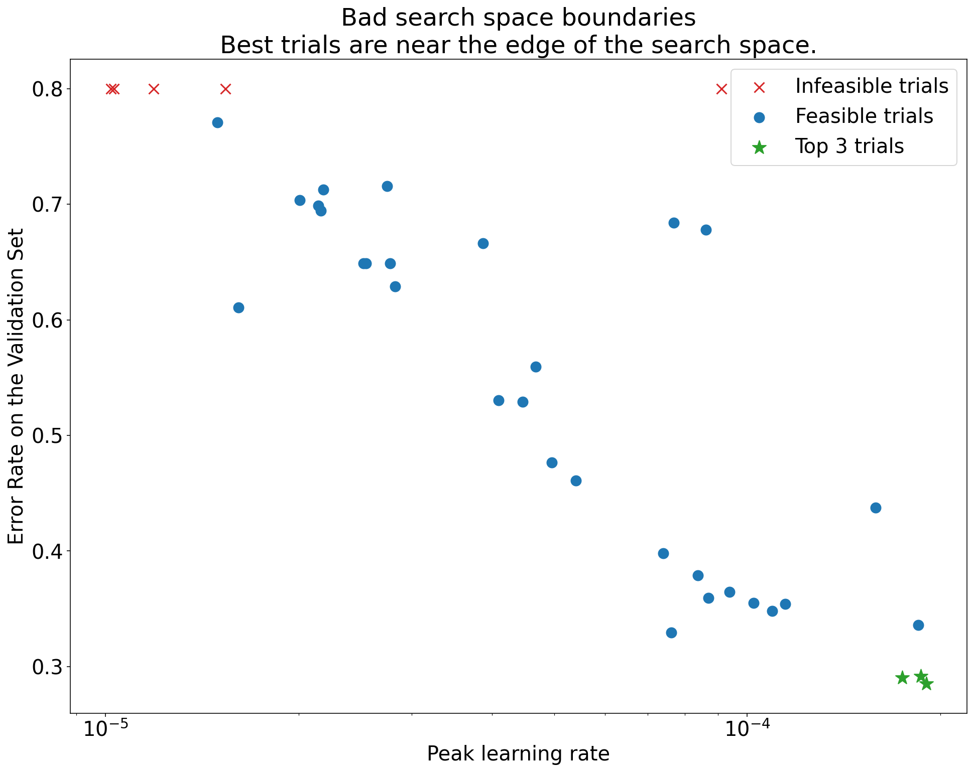
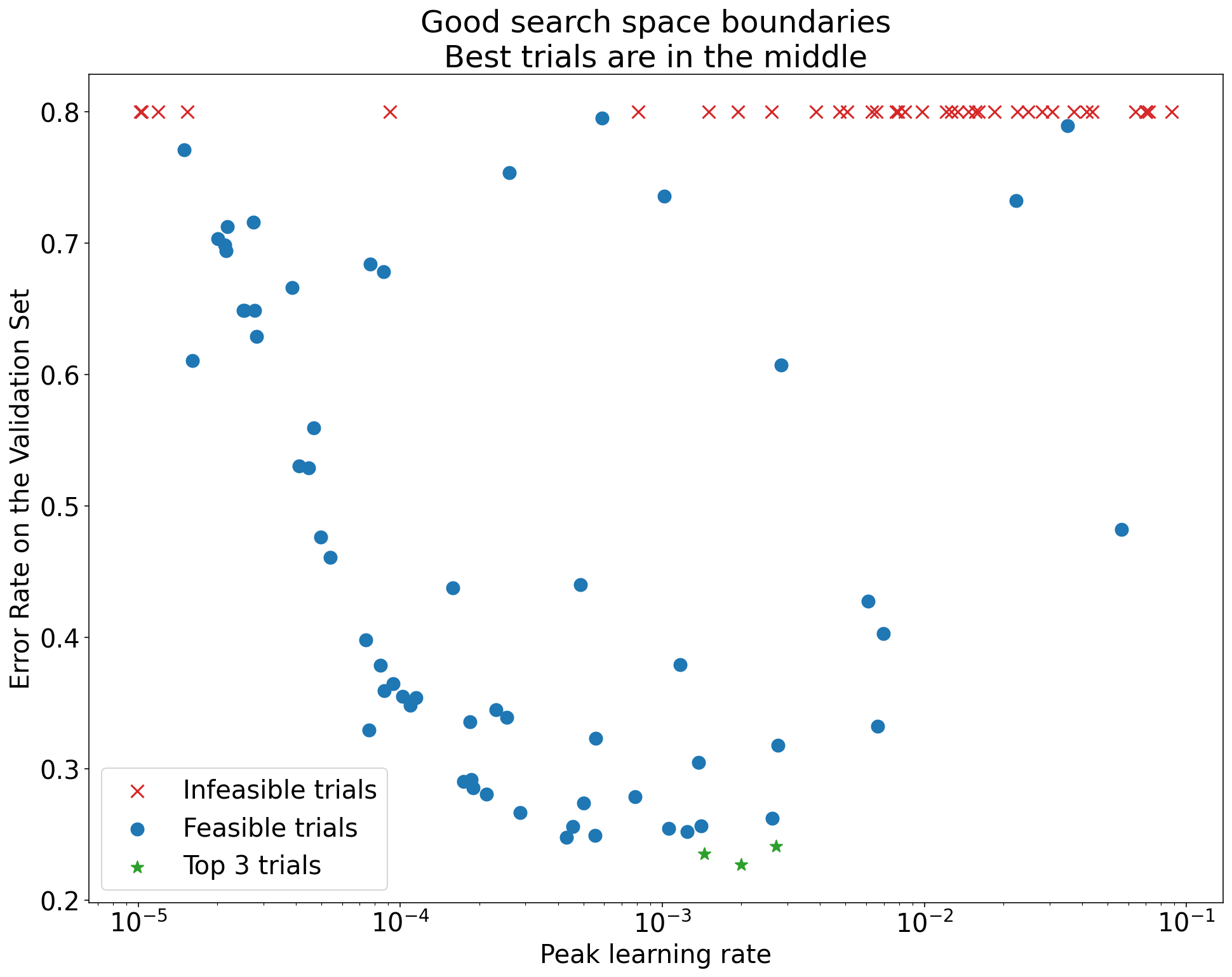
Figure 1: Examples of bad search space boundaries and acceptable search space boundaries.
- The plots in Figure 1 show the error rate (lower is better)
against the initial learning rate. - If the best points cluster towards the edge of a search space (in some
dimension), then the search space boundaries might need to be expanded until
the best observed point is no longer close to the boundary. - Often, a study will include “infeasible” trials that diverge or get very bad
results (marked with red Xs in the above plots).- If all trials are infeasible for learning rates greater than some
threshold value, and if the best performing trials have learning rates
at the edge of that region, the model may suffer from stability issues
preventing it from accessing higher learning
rates.
- If all trials are infeasible for learning rates greater than some
[Click to expand]
- In general,
it can be very difficult to know
if the search space has been sampled densely enough. 🤖 - Running more trials is of course better, but comes at an obvious cost.
- Since it is so hard to know when we have sampled enough, we usually sample
what we can afford and try to calibrate our intuitive confidence from
repeatedly looking at various hyperparameter axis plots and trying to get a
sense of how many points are in the “good” region of the search space.
[Click to expand]
Summary: Examining the training curves is an easy way to identify common
failure modes and can help us prioritize what actions to take next.
- Although in many cases the primary objective of our experiments only
requires considering the validation error of each trial, we must be careful
when reducing each trial to a single number because it can hide important
details about what’s going on below the surface. - For every study, we always look at the training curves (training error
and validation error plotted versus training step over the duration of
training) of at least the best few trials. - Even if this is not necessary for addressing the primary experimental
objective, examining the training curves is an easy way to identify common
failure modes and can help us prioritize what actions to take next. - When examining the training curves, we are interested in the following
questions. - Are any of the trials exhibiting problematic overfitting?
- Problematic overfitting occurs when the validation error starts
increasing at some point during training. - In experimental settings where we optimize away nuisance hyperparameters
by selecting the “best” trial for each setting of the scientific
hyperparameters, we should check for problematic overfitting in at
least each of the best trials corresponding to the
- Problematic overfitting occurs when the validation error starts