


Most contemporary generative models of images, sound and video do not operate directly on pixels or waveforms. They consist of two stages: first, a compact, higher-level latent representation is extracted, and then an iterative generative process operates on this representation instead. How does this work, and why is this approach so popular?
Generative models that make use of latent representations are everywhere nowadays, so I thought it was high time to dedicate a blog post to them. In what follows, I will talk at length about latents as a plural noun, which is the usual shorthand for latent representation. This terminology originated in the concept of latent variables in statistics, but it is worth noting that the meaning has drifted somewhat in this context. These latents do not represent any known underlying physical quantity which we cannot measure directly; rather, they capture perceptually meaningful information in a compact way, and in many cases they are a deterministic nonlinear function of the input signal (i.e. not random variables).
In what follows, I will assume a basic understanding of neural networks, generative models and related concepts. Below is an overview of the different sections of this post. Click to jump directly to a particular section.
- The recipe
- How we got here
- Why two stages?
- Trading off reconstruction quality and modelability
- Controlling capacity
- Curating and shaping the latent space
- The tyranny of the grid
- Latents for other modalities
- Will end-to-end win in the end?
- Closing thoughts
- Acknowledgements
- References
The recipe
The usual process for training a generative model in latent space consists of two stages:
- Train an autoencoder on the input signals. This is a neural network consisting of two subnetworks, an encoder and a decoder. The former maps an input signal to its corresponding latent representation (encoding). The latter maps the latent representation back to the input domain (decoding).
- Train a generative model on the latent representations. This involves taking the encoder from the first stage, and using it to extract latents for the training data. The generative model is then trained directly on these latents. Nowadays, this is usually either an autoregressive model or a diffusion model.
Once the autoencoder is trained in the first stage, its parameters will not change any further in the second stage: gradients from the second stage of the learning process are not backpropagated into the encoder. Another way to say this is that the encoder parameters are frozen in the second stage.
Note that the decoder part of the autoencoder plays no role in the second stage of training, but we will need it when sampling from the generative model, as that will generate outputs in latent space. The decoder enables us to map the generated latents back to the original input space.
Below is a diagram illustrating this two-stage training recipe. Networks whose parameters are learnt in the respective stages are indicated with a (nabla) symbol, because this is almost always done using gradient-based learning. Networks whose parameters are frozen are indicated with a snowflake.
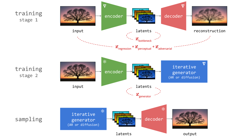
Several different loss functions are involved in the two training stages, which are indicated in red on the diagram:
- To ensure the encoder and decoder are able to convert input representations to latents and back with high fidelity, several loss functions constrain the reconstruction (decoder output) with respect to the input. These usualy include a simple regression loss, a perceptual loss and an adversarial loss.
- To constrain the capacity of the latents, an additional loss function is often applied directly to them during training, although this is not always the case. We will refer to this as the bottleneck loss, because the latent representation forms a bottleneck in the autoencoder network.
- In the second stage, the generative model is trained using its own loss function, separate from those used during the first stage. This is often the negative log-likelihood loss (for autoregressive models), or a diffusion loss.
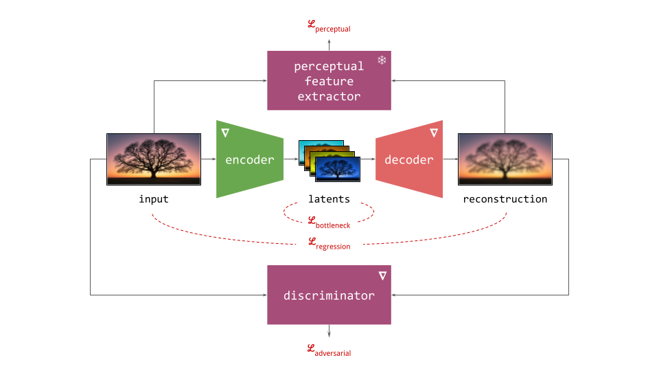
Taking a closer look at the reconstruction-based losses, we have:
- the regression loss, which is sometimes the mean absolute error (MAE) measured in the input space (e.g. on pixels), but more often the mean squared error (MSE).
- the perceptual loss, which can take many forms, but more often than not, it makes use of another frozen pre-trained neural network to extract perceptual features. The loss encourages these features to match between the reconstruction and the input, which results in better preservation of high-frequency content that is largely ignored by the regression loss. LPIPS1 is a popular choice for images.
- the adversarial loss, which uses a discriminator network which is co-trained with the autoencoder, as in generative adversarial networks (GANs)2. The discriminator is trained to tell apart real input signals from reconstructions, and the autoencoder is trained to fool the discriminator into making mistakes. The goal is to improve the realism of the output, even if it means deviating further from the input signal. It is quite common for the adversarial loss to be disabled for some time at the start of training, to avoid instability.
Below is a more elaborate diagram of the first training stage, explicitly showing the other networks which typically play a role in this process.
It goes without saying that this generic recipe is often deviated from in one or more ways, especially for audio and video, but I have tried to summarise the most common ingredients found in most modern practical applications of this modelling approach.
How we got here
The two dominant generative modelling paradigms of today, autoregression and diffusion, were both initially applied to “raw” digital representations of perceptual signals, by which I mean pixels and waveforms. PixelRNN3 and PixelCNN4 generated images one pixel at a time. WaveNet5 and SampleRNN6 did the same for audio, producing waveform amplitudes one sample at a time. On the diffusion side, the original works that introduced7 and established8 9 the modelling paradigm all operated on pixels to produce images, and early works like WaveGrad10 and DiffWave11 generated waveforms to produce sound.
However, it became clear very quickly that this strategy makes scaling up quite challenging. The most important reason for this can be summarised as follows: perceptual signals mostly consist of imperceptible noise. Or, to put it a different way: out of the total information content of a given signal, only a small fraction actually affects our perception of it. Therefore, it pays to ensure that our generative model can use its capacity efficiently, and focus on modelling just that fraction. That way, we can use smaller, faster and cheaper generative models without compromising on perceptual quality.
Latent autoregression
Autoregressive models of images took a huge leap forward with the seminal VQ-VAE paper12. It suggested a practical strategy for learning discrete representations with neural networks, by inserting a vector quantisation bottleneck layer into an autoencoder. To learn such discrete latents for images, a convolutional encoder with several downsampling stages produced a spatial grid of vectors with a 4× lower resolution than the input (along both height and width, so 16× fewer spatial positions), and these vectors were then quantised by the bottleneck layer.
Now, we could generate images with PixelCNN-style models one latent vector at a time, rather than having to do it pixel by pixel. This significantly reduced the number of autoregressive sampling steps required, but perhaps more importantly, measuring the likelihood loss in the latent space rather than pixel space helped avoid wasting capacity on imperceptible noise. This is effectively a different loss function, putting more weight on perceptually relevant signal content, because a lot of the perceptually irrelevant signal content is not present in the latent vectors (see my blog post on typicality for more on this topic). The paper showed 128×128 generated images from a model trained on ImageNet, a resolution that had only been attainable with GANs2 up to that point.
The discretisation was critical to its success, because autoregressive models were known to work much better with discrete inputs at the time. But perhaps even more importantly, the spatial structure of the latents allowed existing pixel-based models to be adapted very easily. Before this, VAEs (variational autoencoders13 14) would typically compress an entire image into a single latent vector, resulting in a representation without any kind of topological structure. The grid structure of modern latent representations, which mirrors that of the “raw” input representation, is exploited in the network architecture of generative models to increase efficiency (through e.g. convolutions, recurrence or attention layers).
VQ-VAE 215 further increased the resolution to 256×256 and dramatically improved image quality through scale, as well as the use of multiple levels of latent grids, structured in a hierarchy. This was followed by VQGAN16, which combined the adversarial learning mechanism of GANs with the VQ-VAE architecture. This enabled a dramatic increase of the resolution reduction factor from 4× to 16× (256× fewer spatial positions compared to pixel input), while still allowing for sharp and realistic reconstructions. The adversarial loss played a big role in this, encouraging realistic decoder output even when it is not possible to closely adhere to the original input signal.
VQGAN became a core technology enabling the rapid progress in generative modelling of perceptual signals that we’ve witnessed in the last five years. Its impact cannot be overestimated – I’ve gone as far as to say that it’s probably the main reason why GANs deserved to win the Test of Time award at NeurIPS 2024. The “assist” that the VQGAN paper provided, kept GANs relevant even after they were all but replaced by diffusion models for the base task of media generation.
IMO VQGAN is why GANs deserve the NeurIPS test of time award. Suddenly our image representations were an order of magnitude more compact. Absolute game changer for generative modelling at scale, and the basis for latent diffusion models.https://t.co/Ochh17IvGx
— Sander Dieleman (@sedielem) November 28, 2024
It is also worth pointing out just how much of the recipe from the previous section was conceived in this paper. The iterative generator isn’t usually autoregressive these days (Parti17, xAI’s recent Aurora model and, apparently, OpenAI’s GPT-4o are notable exceptions), and the quantisation bottleneck has been replaced, but everything else is still there. Especially the combination of a simple regression loss, a perceptual loss and an adversarial loss has stubbornly persisted, in spite of its apparent complexity. This kind of endurance is rare in a fast-moving field like machine learning – perhaps rivalled only by that of the largely unchanged Transformer architecture18 and the Adam optimiser19!
(While discrete representations played an essential role in making latent autoregression work at scale, I wanted to point out that autoregression in continuous space has also been made to work well recently20 21.)
Latent diffusion
With latent autoregression gaining ground in the late 2010s, and diffusion models breaking through in the early 2020s, combining the strengths of both approaches was a natural next step. As with many ideas whose time has come, we saw a string of concurrent papers exploring this topic hit arXiv around the same time, in the second half of 202122 23 24 25 26. The most well-known of these is Rombach et al.’s High-Resolution Image Synthesis with Latent Diffusion Models26, who reused their previous VQGAN work16 and swapped out the autoregressive Transformer for a UNet-based diffusion model. This formed the basis for the Stable Diffusion models. Other works explored similar ideas, albeit at a smaller scale24, or for modalities other than images22.
It took a little bit of time for the approach to become mainstream. Early commercial text-to-image models made use of so-called resolution cascades, consisting of a base diffusion model that generates low-resolution images directly in pixel space, and one or more upsampling diffusion models that produce higher-resolution outputs conditioned on lower-resolution inputs. Examples include DALL-E 2 and Imagen 2. After Stable Diffusion, most moved to a latent-based approach (including DALL-E 3 and Imagen 3).
An important difference between autoregressive and diffusion models is the loss function used to train them. In the autoregressive case, things are relatively simple: you just maximise the likelihood (although other things have been tried as well27). For diffusion, things are a little more interesting: the loss is an expectation over all noise levels, and the relative weighting of these noise levels significantly affects what the model learns (for an explanation of this, see my previous blog post on noise schedules, as well as my blog post about casting diffusion as autoregression in frequency space). This justifies an interpretation of the typical diffusion loss as a kind of perceptual loss function, which puts more emphasis on signal content that is more perceptually salient.
At first glance, this makes the two-stage approach seem redundant, as it operates in a similar way, i.e. filtering out perceptually irrelevant signal content, to avoid wasting model capacity on it. If we can rely on the diffusion loss to focus only on what matters perceptually, why do we need a separate representation learning stage to filter out the stuff that doesn’t? These two mechanisms turn out to be quite complementary in practice however, for two reasons:
- The way perception works at small and large scales, especially in the visual domain, seems to be fundamentally different – to the extent that modelling texture and fine-grained detail merits separate treatment, and an adversarial approach can be more suitable for this. I will discuss this in more detail in the next section.
- Training large, powerful diffusion models is inherently computationally intensive, and operating in a more compact latent space allows us to avoid having to work with bulky input representations. This helps to reduce memory requirements and speeds up training and sampling.
Some early works did consider an end-to-end approach, jointly learning the latent representation and the diffusion prior23 25, but this didn’t really catch on. Although avoiding sequential dependencies between multiple stages of training is desirable from a practical perspective, the perceptual and computational benefits make it worth the hassle.
Why two stages?
As discussed before, it is important to ensure that generative models of perceptual signals can use their capacity efficiently, as this makes them much more cost-effective. This is essentially what the two-stage approach accomplishes: by extracting a more compact representation that focuses on the perceptually relevant fraction of signal content, and modelling that instead of the original representation, we are able to make relatively modestly sized generative models punch above their weight.
The fact that most bits of information in perceptual signals don’t actually matter perceptually is hardly a new observation: it is also the key idea underlying lossy compression, which enables us to store and transmit these signals at a fraction of the cost. Compression algorithms like JPEG and MP3 exploit the redundancies present in signals, as well as the fact that our audiovisual senses are more sensitive to low frequencies than to high frequencies, to represent perceptual signals with far fewer bits. (There are other perceptual effects that play a role, such as auditory masking for example, but non-uniform frequency sensitivity is the most important one.)
So why don’t we use these lossy compression techniques as a basis for our generative models then? This is not a bad idea, and several works have used these algorithms, or parts of them, for this purpose28 29 30. But a very natural reflex for people working on generative models is to try to solve the problem with more machine learning, to see if we can do better than these “handcrafted” algorithms.
It’s not just hubris on the part of ML researchers, though: there is actually a very good reason to use learned latents, instead of using these pre-existing compressed representations. Unlike in the compression setting, where smaller is better, and size is all that matters, the goal of generative modelling also imposes other constraints: some representations are easier to model than others. It is crucial that some structure remains in the representation, which we can then exploit by endowing the generative model with the appropriate inductive biases. This requirement creates a trade-off between reconstruction quality and modelability of the latents, which we will investigate in the next section.
An important reason behind the efficacy of latent representations is how they lean in to the fact that our perception works differently at different scales. In the audio domain, this is readily apparent: very rapid changes in amplitude result in the perception of pitch, whereas changes on coarser time scales (e.g. drum beats) can be individually discerned. Less well-known is that the same phenomenon also plays an important role in visual perception: rapid local fluctuations in colour and intensity are perceived as textures. A while back, I tried to explain this on Twitter, and I will paraphrase that explanation here:
One way to think of it is texture vs. structure, or sometimes people call this stuff vs. things.
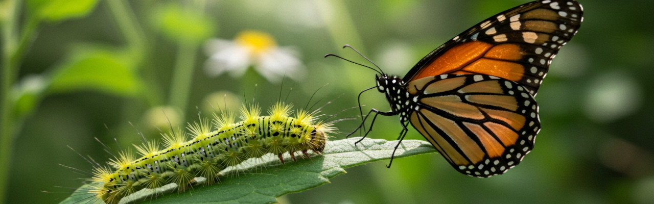
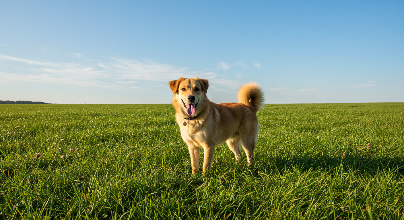
In an image of a dog in a field, the grass texture (stuff) is high-entropy, but we are bad at perceiving differences between individual realisations of this texture, we just perceive it as “grass”, in an uncountable sense. We do not need to individually observe each blade of grass to determine that what we’re looking at is a field.
If the realisation of this texture is subtly different, we often cannot tell, unless the images are layered directly on top of each other. This is a fun experiment to try with an adversarial autoencoder: when comparing an original image and its reconstruction side by side, they often look identical. But layering them on top of each other and flipping back and forth often reveals just how different the images are, especially in areas with a lot of texture.
For objects (things) on the other hand, like the dog’s eyes, for example, differences of a similar magnitude would be immediately obvious.
A good latent representation will make abstraction of texture, but try to preserve structure. That way, the realisation of the grass texture in the reconstruction can be different than the original, without it noticeably affecting the fidelity of the reconstruction. This enables the autoencoder to drop a lot of modes (i.e. other realisations of the same texture) and represent the presence of this texture more compactly in its latent space.
This in turn should make generative modelling in the latent space easier as well, because it can now model the absence/presence of a texture, rather than having to capture all the entropy associated with that texture.
Because of the dramatic improvements in efficiency that the two-stage approach offers, we seem to be happy to put up with the additional complexity it entails – at least, for now. This increased efficiency results in faster and cheaper training runs, but perhaps more importantly, it can greatly accelerate sampling as well. With generative models that perform iterative refinement, this significant cost reduction is of course very welcome, because many forward passes through the model are required to produce a single sample.
Trading off reconstruction quality and modelability
The difference between lossy compression and latent representation learning is worth exploring in more detail. One can use machine learning for both, although most lossy compression algorithms in widespread use today do not. These algorithms are typically rooted in rate-distortion theory, which formalises and quantifies the relationship between the degree to which we are able to compress a signal (rate), and how much we allow the decompressed signal to deviate from the original (distortion).
For latent representation learning, we can extend this trade-off by introducing the concept of modelability or learnability, which characterises how challenging it is for generative models to capture the distribution of this representation. This results in a three-way rate-distortion-modelability trade-off, which is closely related to the rate-distortion-usefulness trade-off discussed by Tschannen et al. in the context of representation learning31. (Another popular way to extend this trade-off in a machine learning context is the rate-distortion-perception trade-off32, which explicitly distinguishes reconstruction fidelity from perceptual quality. To avoid overcomplicating things, I will not make this distinction here, instead treating distortion as a quantity measured in a perceptual space, rather than input space.)
It’s not immediately obvious why this is even a trade-off at all – why is modelability at odds with distortion? To understand this, consider how lossy compression algorithms operate: they take advantage of known signal structure to reduce redundancy. In the process, this structure is often removed from the compressed representation, because the decompression algorithm is able to reconstitute it. But structure in input signals is also exploited extensively in modern generative models, in the form of architectural inductive biases for example, which take advantage of signal properties like translation equivariance or specific characteristics of the frequency spectrum.
If we have an amazing algorithm that efficiently removes almost all redundancies from our input signals, we are making it very difficult for generative models to capture the unstructured variability that remains in the compressed signals. That is completely fine if compression is all we are after, but not if we want to do generative modelling. So we have to strike a balance: a good latent representation learning algorithm will detect and remove some redundancy, but keep some signal structure as well, so there is something left for the generative model to work with.
A good example of what not to do in this setting is entropy coding, which is actually a lossless compression method, but is also used as the final stage in many lossy schemes (e.g. Huffman coding in JPEG/PNG, or arithmetic coding in H.265). Entropy coding algorithms reduce redundancy by assigning shorter representations to frequently occurring patterns. This doesn’t remove any information at all, but it destroys structure. As a result, small changes in input signals could lead to much larger changes in the corresponding compressed sig